MD-COAS — Motion Planning with Model-Based Diffusion via Constraint Optimization and Adaptive Scheduling

The question

How can a generative planner preserve useful exploration while enforcing difficult constraints, without spending the same correction effort at every denoising step?

Demonstrations

Candidate trajectories from the same L10 / seed 8 planning case.
Source excerpt rescaled to 6.0 seconds; looped, silent; not real-time execution or latency evidence.

An arm executes obstacle-avoidance motion in the D3IL environment.
Source excerpt rescaled to 6.0 seconds; looped, silent; not real-time execution or latency evidence.

How it works

Keep imperfect samples informative

An inexact Augmented Lagrangian soft feasibility prior gives continuous weight to mildly infeasible candidates. Their constraint information can still guide the next update instead of disappearing behind a hard feasible-or-infeasible indicator.

Correct the full control sequence

A Convex Feasible Set projection constructs local constraint approximations and solves a structured quadratic program over the control sequence. Re-rolling the corrected controls through the dynamics preserves the connection between planned motion and the model.

Adapt enforcement during denoising

Constraint residuals adjust the soft-prior multipliers and penalties. A compute-aware primal–dual schedule also controls projection frequency, inner iterations, and active constraints, concentrating correction effort where it is needed.

Results

Paper results evaluate constraint optimization and adaptive scheduling on ten 2D difficulty levels and a 7-DoF arm obstacle-avoidance task.

Arm avoidance

100% safe success

Zero reported violations at all three tested obstacle radii; 5 random seeds and 20 trajectory candidates per seed at each level.

2D constrained maps

0.98–1.00 SSR

Safe & Success Rate reported in the result heatmap for Easy and Constrained map families, L1–L6. The more difficult non-convex Union Maps, L7–L10, achieve approximately 50% SSR.

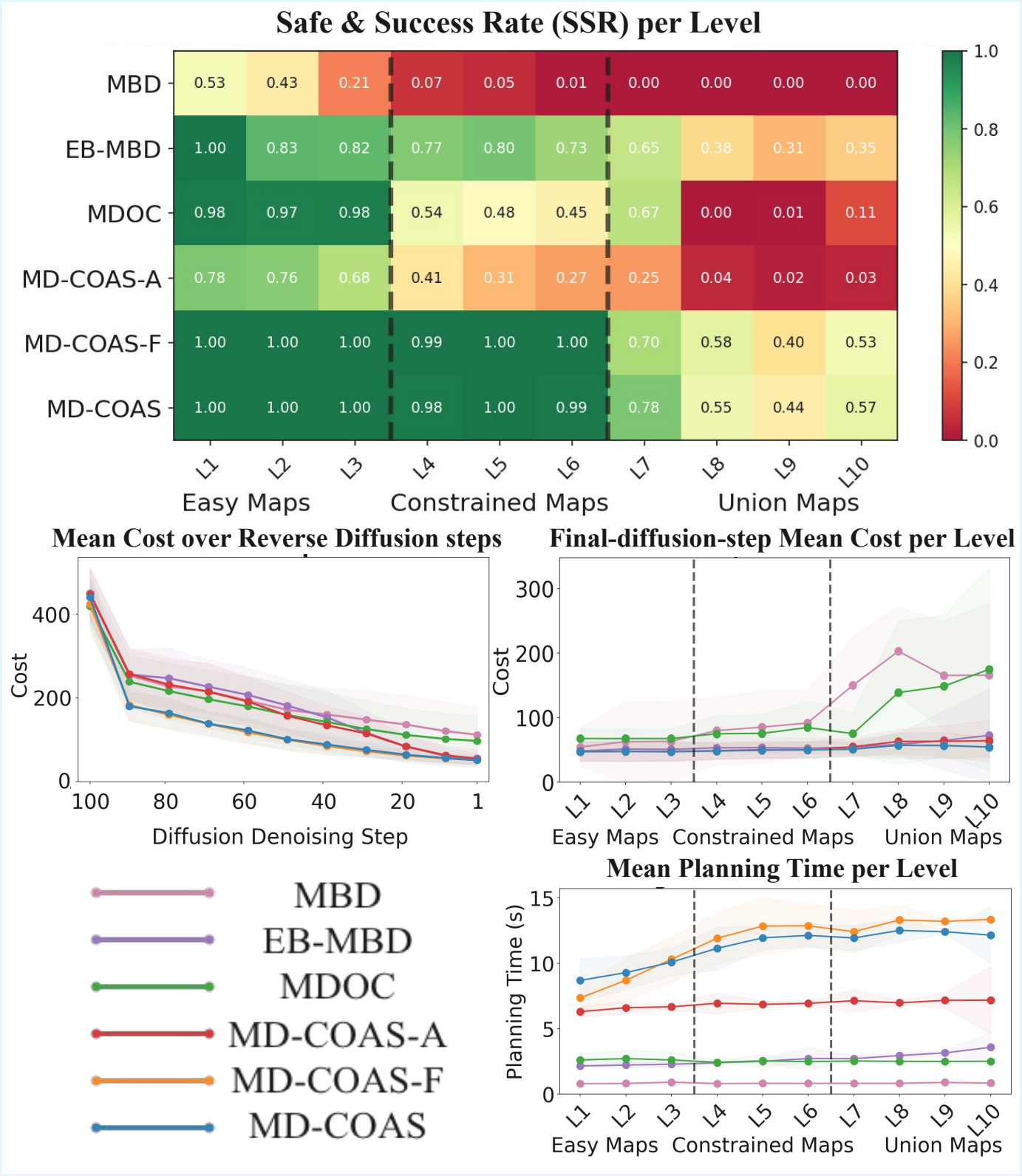
Original paper heatmap of safe and success rate at levels L1 to L10, with cost convergence, final cost, runtime, and all method legends. — Safety, cost, and runtime across 2D maps
Full resolution ↗
Safe & Success Rate at each difficulty level, followed by cost over reverse-diffusion steps, final cost, and planning time. Each level uses 10 random seeds and 20 trajectory modes per seed. Shaded regions show one standard deviation. MD-COAS-A and MD-COAS-F are ablations; the full method is the MD-COAS row.
Figure 3 · Paper ↗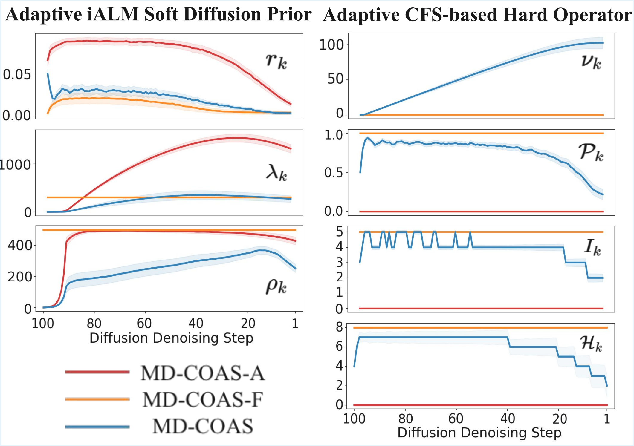

Original paper plots of the residual-driven augmented Lagrangian duals and adaptive CFS projection scheduling across reverse diffusion. — How safety effort adapts during denoising
Full resolution ↗
Safety-enforcement variables over reverse-diffusion steps, averaged across all 2D levels and seeds. Left: iALM dual and penalty updates driven by the feasibility residual. Right: CFS projection probability, iteration budget, active-set size, and compute dual. The plot compares the full method with two ablations.
Figure 4 · Paper ↗

7-DoF arm obstacle avoidance

Quantitative results as obstacle radius increases. SSR is Safe & Success Rate (↑); V is violation rate (% ↓); T is planning time (↓); P is path length (↓). Means are reported across seeds, with path length averaged over safe and successful trajectories.

MD-COAS: 7-DoF arm obstacle avoidance. Quantitative results as obstacle radius increases. SSR is Safe & Success Rate (↑); V is violation rate (% ↓); T is planning time (↓); P is path length (↓). Means are reported across seeds, with path length averaged over safe and successful trajectories.
	Obstacle radius = 0.03				Obstacle radius = 0.04				Obstacle radius = 0.05
Method	SSR ↑	V (%) ↓	T ↓	P ↓	SSR ↑	V (%) ↓	T ↓	P ↓	SSR ↑	V (%) ↓	T ↓	P ↓
SafeDiffuser	0.45	1.30	5.49 ± 0.20	1.57 ± 0.05	0.35	2.68	11.53 ± 1.30	1.56 ± 0.05	0.30	4.40	11.18 ± 0.10	1.54 ± 0.03
DPCC-C	0.75	0.78	1528.91 ± 571.70	1.32 ± 0.39	0.54	1.44	2561.96 ± 1818.70	1.51 ± 0.53	0.64	2.10	3460.31 ± 1568.70	1.44 ± 0.40
EB-MBD	0.98	0.00	4.37 ± 2.00	1.01 ± 0.05	0.91	0.00	4.02 ± 0.60	1.02 ± 0.05	0.82	0.00	4.06 ± 0.60	1.01 ± 0.06
MDOC	1.00	0.00	5.65 ± 1.90	0.89 ± 0.04	0.99	0.04	4.90 ± 0.60	0.88 ± 0.04	0.73	0.02	4.87 ± 0.70	0.90 ± 0.04
MD-COAS (ours)	1.00	0.00	13.53 ± 2.90	0.99 ± 0.04	1.00	0.00	13.98 ± 2.10	0.99 ± 0.05	1.00	0.00	14.87 ± 2.10	1.00 ± 0.07

Five random seeds and 20 trajectory modes per seed at each obstacle radius: 100 modes per method and level. End-effector radius is fixed at 0.01.

Experimental protocol and metric definitions

± values are standard deviations, rendered from the original right-superscript notation. The paper reports no standard deviations for SSR or V.

The source table does not specify physical units for T, P, or obstacle radius; these are reproduced as reported.

CFS projection is applied to all unweighted trajectory samples. The paper reports a trade-off between planning performance and computation time.

Hardware: NVIDIA RTX A6000 (48 GB) and 9 CPU cores; CFS projections use jaxopt.

Table I · Paper ↗

Scope & trade-offs

Training-free single-robot planning with known dynamics, evaluated on randomized 2D obstacle maps and a D3IL 7-DoF arm avoidance task. The arm plans in joint space while its end-effector remains on a 2D workspace plane.

Full-sample CFS projection has a computational cost. MD-COAS is slower than MDOC in the reported 7-DoF table; adaptive scheduling improves efficiency relative to uniformly applied correction rather than guaranteeing a speedup over every baseline.

The hardest non-convex 2D maps remain challenging; the paper does not report universal success or safety across arbitrary environments.

This paper evaluates single-robot tasks. Richer dynamics and multi-robot coordination are future directions, not demonstrated extensions.

The next question

MD-COAS adapts how strongly and how often feasibility is enforced. 2GO asks how active constraint geometry can also shape the direction of refinement and the stochastic exploration itself, extending the story to constrained locomotion.

Citation

@inproceedings{he2026mdcoas,
  title={Motion Planning with Model-Based Diffusion via Constraint Optimization and Adaptive Scheduling},
  author={He, Zhilin and Li, Bowei and Dou, Jianlin and Zhang, Yuner and Liu, Changliu},
  booktitle={2026 IEEE/RSJ International Conference on Intelligent Robots and Systems (IROS)},
  year={2026}
}

Figures and tables reproduce the manuscript's reported experiments. Demonstrations are representative runs; experimental populations and metrics are specified with each table.

MD-COASBalance exploration, feasibility, and compute.